Simulate flow in a static mixer

This basic example shows how to launch PyCFX and then set up, run, and postprocess the CFX Static Mixer tutorial case in PyCFX.

Model overview

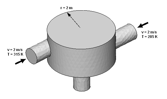
This example simulates a static mixer with two inlet pipes delivering water into a mixing vessel. The water exits through an outlet pipe.

Water enters through both pipes at the same rate but at different temperatures. The first entry is at a rate of 2 m/s and a temperature of 315 K. The second entry is at a rate of 2 m/s and a temperature of 285 K. The mixer radius is 2 m.

Workflow tasks

The static mixer example guides you through these tasks:

• Set up a basic case in a PreProcessing session (CFX-Pre).

• Run the CFX-Solver.

• Perform basic postprocessing in CFD-Post.

Initial setup

Perform required imports

Perform the required imports. It is assumed that the ansys-cfx-core package has been installed.

import os

import ansys.cfx.core as pycfx
from ansys.cfx.core import examples

Download required files

mesh_file_name = examples.download_file(
    "StaticMixerMesh.gtm",
    "pycfx/static_mixer",
    save_path=os.getcwd(),
)

Preprocessing

Start a PreProcessing session (CFX-Pre) and create a new case

pypre = pycfx.PreProcessing.from_install()
pypre.file.new_case()

Import a mesh

The StaticMixerMesh.gtm mesh file should already have been downloaded to the current working directory earlier in this script.

pypre.file.import_mesh(file_name=mesh_file_name)

Set up the domain

A default domain is created automatically when a new case is created.

default_domain = pypre.setup.flow["Flow Analysis 1"].domain["Default Domain"]
default_domain.fluid_definition["Fluid 1"].material = "Water"
default_domain.domain_models.reference_pressure.reference_pressure = "1 [atm]"
default_domain.fluid_models.heat_transfer_model.option = "Thermal Energy"
default_domain.fluid_models.turbulence_model.option = "k epsilon"

Set up the boundary conditions

Add the first inlet boundary, specifying each setting in turn.

default_domain.boundary["in1"] = {}
in1 = default_domain.boundary["in1"]
in1.boundary_type = "INLET"
in1.location = "in1"
in1.boundary_conditions.mass_and_momentum.option = "Normal Speed"
in1.boundary_conditions.mass_and_momentum.normal_speed = "2 [m s^-1]"
in1.boundary_conditions.heat_transfer.static_temperature = "315 [K]"

Add the second inlet boundary by duplicating the first.

in1_state = default_domain.boundary["in1"].get_state()
default_domain.boundary["in2"] = in1_state
in2 = default_domain.boundary["in2"]
in2.location = "in2"
in2.boundary_conditions.heat_transfer.static_temperature = "285 [K]"

Add the outlet boundary.

pypre.setup.flow["Flow Analysis 1"].domain["Default Domain"].boundary["out"] = {}
out = pypre.setup.flow["Flow Analysis 1"].domain["Default Domain"].boundary["out"]
out.boundary_type = "OUTLET"
out.location = "out"
out.boundary_conditions.mass_and_momentum.option = "Average Static Pressure"
out.boundary_conditions.mass_and_momentum.relative_pressure = "0 [Pa]"

Set up the solver

Configure the solver control settings.

solver_control = pypre.setup.flow["Flow Analysis 1"].solver_control
solver_control.advection_scheme.option = "Upwind"
solver_control.convergence_control.timescale_control = "Physical Timescale"
solver_control.convergence_control.physical_timescale = "2 [s]"

Set up the CFX-Solver to run in parallel using execution control.

exec_control = pypre.setup.simulation_control.execution_control
exec_control.solver_step_control.parallel_environment.start_method = "Intel MPI Local Parallel"
exec_control.solver_step_control.parallel_environment.maximum_number_of_processes = 2

Check for errors

Check for physics messages to ensure the setup is consistent and no required settings are missing.

physics_messages = pypre.setup.get_physics_messages(severity="All")
if physics_messages:
    print(f"Physics messages: {physics_messages}")

Write the CFX-Solver input file

This example uses a file-based workflow, where each of the three PyCFX components (PreProcessing, Solver, and PostProcessing) are run independently, with each component being initialized by a file written by the previous component where possible. This allows each component to be run separately, potentially on a different machine configuration, at a different time, or from a different Python session. In contrast, the Fourier Transformation Blade Flutter case example shows a workflow where the PyCFX components interact more directly.

Write the CFX-Solver input file and close the preprocessing session.

solver_input_file_name = "static_mixer.def"
pypre.file.write_solver_input_file(file_name=solver_input_file_name)
pypre.exit()

Run the solver

Start a Solver session and launch the CFX-Solver

Launch the CFX-Solver using the execution control settings applied in the preprocessing session. Only local CFX-Solver runs are supported.

pysolve = pycfx.Solver.from_install(solver_input_file_name=solver_input_file_name)
pysolve.solution.start_run()

Wait for the run to complete

Wait for the run to complete and determine the results file name.

pysolve.solution.wait_for_run()
results_file = pysolve.solution.get_results_file_name()
pysolve.exit()

Postprocessing

Start a PostProcessing session (CFD-Post)

Start CFD-Post and load the results.

pypost = pycfx.PostProcessing.from_install(results_file_name=results_file)

Find the name of the case object that is automatically created.

case_names = pypost.results.data_reader.case.get_object_names()
if case_names:
    current_case = case_names[0]
else:
    raise RuntimeError("Loading results failed; no cases defined.")

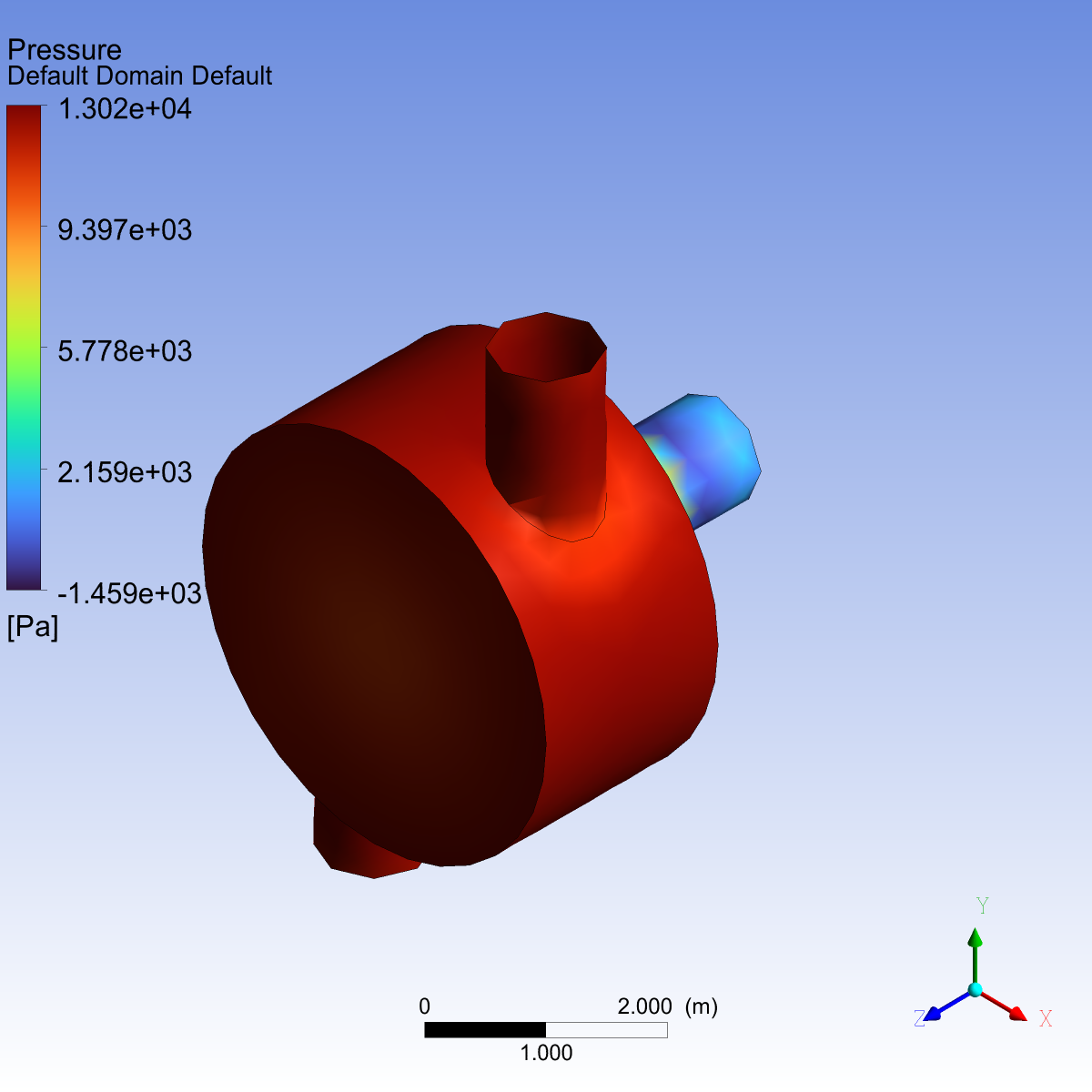
Plot contours on one of the boundaries

pypost.results.data_reader.case[current_case] = {
    "boundary": {
        "Default Domain Default": {
            "colour_mode": "Variable",
            "colour_variable": "Pressure",
            "draw_contours": True,
        }
    }
}
current_case = pypost.results.data_reader.case[current_case]
default_boundary = current_case.boundary["Default Domain Default"]
default_boundary.show(view="/VIEW:View 1")

Create an image

Set up the image.

hardcopy = pypost.results.hardcopy
hardcopy.hardcopy_format = "png"
hardcopy.image_height = 1200
hardcopy.image_width = 1200
hardcopy.use_screen_size = False

Save the image. Hide the boundary again so that it is not visible in subsequent images.

pypost.file.save_picture(file_name="static_mixer_boundary.png")
default_boundary.hide()

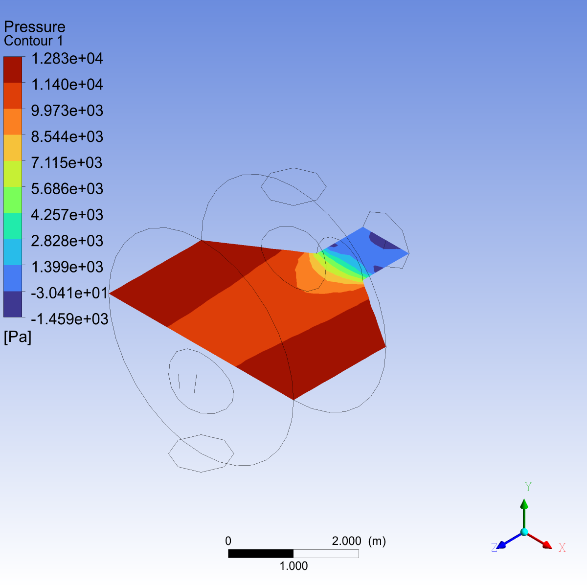
Create a plane

By default, the plane geometry recalculates every time a setting is modified. When modifying several settings sequentially, suspend the plane object to avoid unnecessary intermediate calculations. Unsuspend the plane after completing the setup to reflect the latest settings.

pypost.results.plane["Plane 1"] = {}
plane = pypost.results.plane["Plane 1"]
plane.suspend()
plane.option = "ZX Plane"
plane.plane_type = "Slice"
plane.unsuspend()

Create a contour

Create a contour on the previously defined plane and save the image. Supplying all the settings at once by using a dictionary is another way to avoid unnecessary intermediate calculations.

pypost.results.contour["Contour 1"] = {
    "colour_variable": "Pressure",
    "location_list": "/PLANE:Plane 1",
    "number_of_contours": 11,
    "contour_range": "Local",
    "draw_contours": True,
    "fringe_fill": True,
}
contour = pypost.results.contour["Contour 1"]
contour.show(view="/VIEW:View 1")
pypost.file.save_picture(file_name="static_mixer_contour.png")
contour.hide()

Set up an expression

Set up and evaluate an expression.

pypost.results.library.cel.expressions = {
    "Temperature Difference": {"definition": "maxVal(Temperature)@out - minVal(Temperature)@out"}
}
expressions = pypost.results.library.cel.expressions
print(f"Expressions list: {expressions.list()}")
print(f"Expression definitions: \n{expressions.list_properties()}")
temperature_difference = expressions["Temperature Difference"].evaluate()
print(f"Temperature difference: {temperature_difference}")

Close the postprocessing session

pypost.exit()